VeridianCodex

Understanding how we think, act, and grow is key to unlocking human potential. Our projects dive into the science of decision-making and behavior, offering simple experimental designs, statistical tools, and real-world insights for everyone to use—free of charge. Drawing from personal experiences and rigorous research, we share practical resources to support your professional and personal development, no matter your field.

Control vs. Experimental Groups: The Foundation of Research

At the heart of every experiment lies a control group—the baseline that stays unchanged—and experimental groups, where we test new variables. Think of a placebo in a medical trial, or comparing plant growth with different fertilizers. From exploring how coffee sharpens reaction times to studying art's impact on mental health, these methods help us uncover what drives change. An experiment needs to be replicable if others decide to redo the study, results must be consistent for a phenomenon to be considered scientifically valid and identifies biases and possible errors. This provides progress for each field and encompasses the world building organism we are.

Dive into our examples and resources to design your own experiments and discover the science behind everyday decisions.

Dependent and Independent Variables

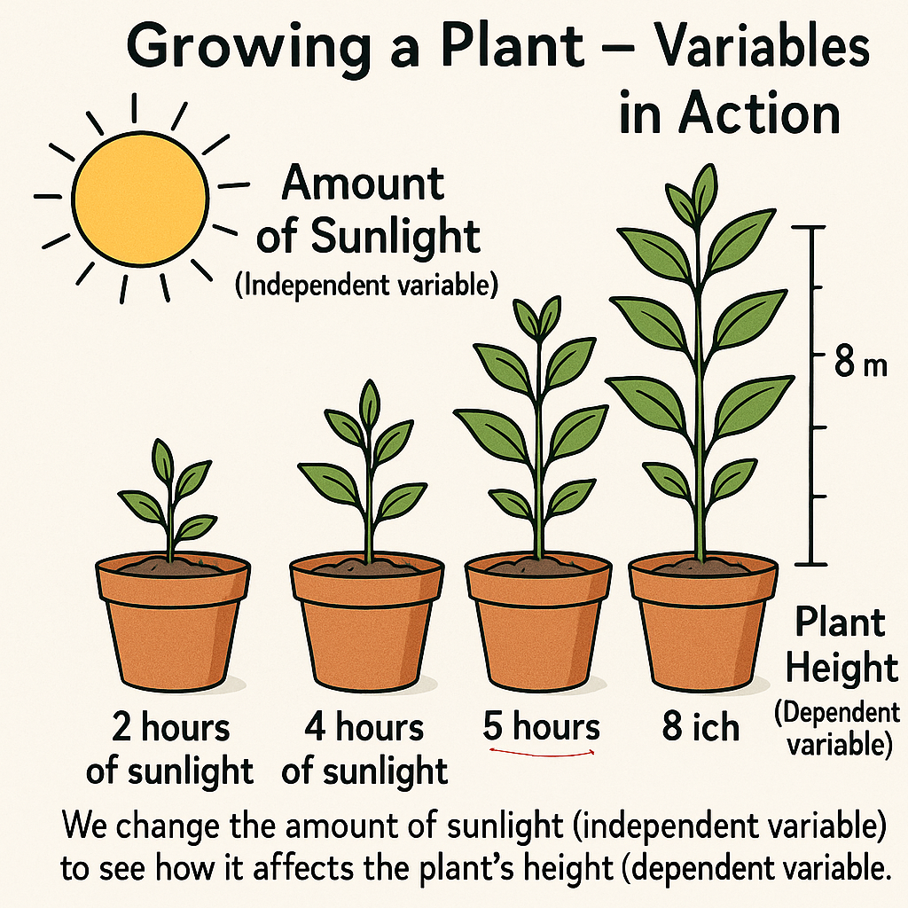
Experiments hinge on two key elements: dependent variables (the outcomes you measure) and independent variables (the factors you control). For example, in a plant growth study, the height of the plant is the dependent variable—it depends on what you change, like the amount of sun, water or type of soil, which are independent variables. Understanding these building blocks helps you craft experiments that reveal cause and effect. Researchers also tackle confounding variables—external factors like weather or mood—that could skew results, ensuring clear, reliable insights.

Quantitative, Qualitative, and Mixed Methods

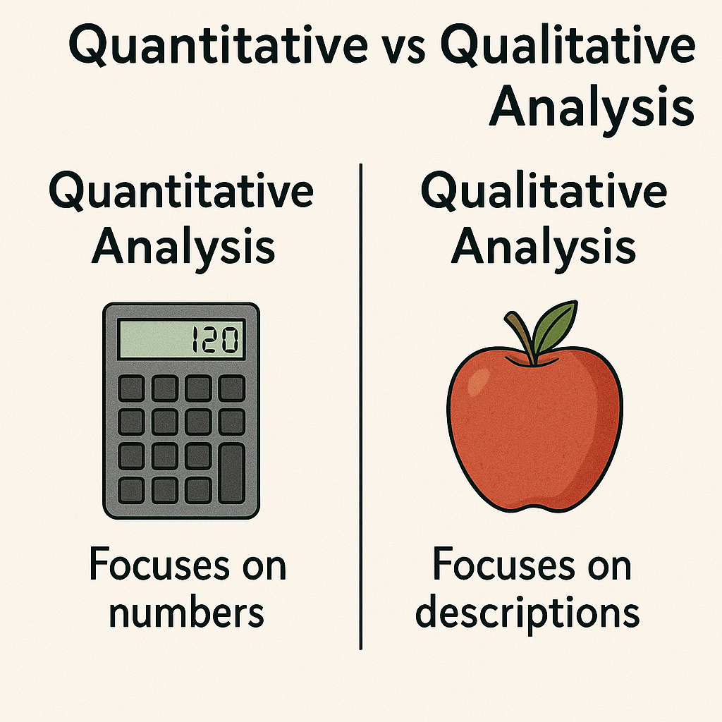
Research comes in different forms. Quantitative methods focus on numbers and measurable data, like tracking reaction times or plant growth rates, to uncover patterns and test hypotheses. Qualitative methods dive into experiences and behaviors, using interviews or observations to explore. Mixed methods combine both, blending hard data with rich narratives for a fuller picture.

Design Paradigms

Between-Subject Design

In this setup, each participant or test subject experiences only one condition. For example, to study plant health, one group of plants might get a new fertilizer, while another gets none. By comparing the groups, you can spot differences caused by the fertilizer. This design is great for isolating specific effects.

Within-Subject Design

Here, every participant experiences all conditions, allowing you to compare effects within the same subject. Imagine testing reaction times before and after drinking coffee on the same person. This approach minimizes individual differences, making it easier to pinpoint the variable's impact.

Example of Simple Experiments

Between Subject t-test

Let us compare the mean scores between 2 groups of 25 individuals each by using a simple between subject t-test.

Let us say group A scored 80 mean score and 10 standard deviation, whereas group b scores 85 mean score and a standard deviation of 12.

Calculate SP:

T-test:

Null Hypothesis vs. Alternative Hypothesis

In research, the null hypothesis (H0) assumes no effect or no difference between groups, serving as the default position to test against—for example, stating that a new fertilizer has no impact on plant growth. The alternative hypothesis (H1) proposes that there is an effect or difference, like claiming the fertilizer A does boost growth. By analyzing data, such as through a t-test, researchers decide whether to reject the null hypothesis in favor of the alternative or fail to reject it, revealing whether the tested variable makes a significant impact.

The p-value is a statistical measure that helps determine the significance of your research findings. A small p-value (typically less than 0.05) suggests strong evidence against the null hypothesis, indicating that the observed effect—such as a difference in group means—is unlikely due to chance alone. For example, in a t-test comparing two groups, a p-value of 0.03 would support rejecting the null hypothesis. In the example above, the measurements were found to be non-significant.

Hypothesis tests can be conducted using either a one-tailed or two-tailed approach. One-tailed tests are directional, used to determine whether a variable specifically increases or decreases an outcome in the experimental group. In contrast, two-tailed tests assess whether there is any significant difference between groups, regardless of the direction of the effect.

Type I and Type II Errors

Type I and Type II errors are two possible mistakes in hypothesis testing. A Type I error occurs when the null hypothesis is incorrectly rejected, (false positive) concluding there is an effect when there isn't one. In contrast, a Type II error happens when the null hypothesis is not rejected despite being false, (false negative) failing to detect a real effect. Both errors highlight the importance of carefully balancing significance levels and statistical power in experimental design.

Calculating p value

The t-value (t = -1.60)

Degrees of freedom (df): (Refers to the independent pieces of information that are free to vary, meaning values that are determined by previous observations and cannot "vary". For example, if you choose 5 integrers that sum up to 100, then the 5th numbers on the list will always be determined by the sum of the previous 4, thus cannot vary.)

For df = 48:

• The critical t-value for a two-tailed test at alpha = 0.10 is approximately 1.677.
• The critical t-value for alpha = 0.20 is approximately 1.299.

Since t = 1.600 falls between 1.299 and 1.677, the two-tailed p-value is between 0.10 and 0.20. Using interpolation or statistical software for precision, the p-value for t = 1.600, df = 48, two-tailed, is approximately 0.116, hence non-significant. Even though there was a small difference between the two mean values in the example, the test has shown that there was no meaningful difference between them.

A critical test value is a threshold used in t analyses to determine whether to reject a null hypothesis or not. You can read more information and save the table for future reference here.

Example on how to report the results:

The site will discuss statistical analysis but please note that it is much more convenient and professional to use statistical analysis software such as SPSS, R or JASP to conduct your analysis. The example showcased here is for introductory purposes only in order to complement future content of the site.